Forced vs unforced: which should be used?
After the object detections in multiple filters are merged, the measurement algorithms are run for each filter separately allowing object centroids and shapes to vary by a small amount. These unforced measurements are suited for studies of object properties in a specific filter, e.g., (approximate) total magnitude of an object in the i-band. For colors, however, it is better to use the forced measurements in which common object centroids and shape parameters are used in all the filters.
Which photometry should be used, PSF, Kron, or cModel?
If you are interested in colors of objects, it is good to use photometry that explicitly takes into account the PSF in the measurement such as PSF photometry and CModel photometry because each filter has a different seeing size in the coadds (PSF is not equalized between the filters in the coadds). For point sources, PSF photometry is the method of choice. For extended sources, one can use CModel. If you are not sure if your objects are extended, or if you work on both compact and extended sources, CModel is the best choice. CModel asymptotically approaches PSF photometry for compact sources and can be used for both compact and extended sources.
However, the deblender tends to fail in crowded areas. The deblender failure affects the photometry and one is advised to use the PSF-matched aperture photometry (a.k.a. afterburner photometry) in such regions. It gives good colors even for isolated objects, and thus it is a good alternative to CModel. However, it is missing light outside the aperture and should not be used for total magnitudes.
If you are interested in measurements in a single-band, Kron photometry is a well-tested method to capture a large fraction of object light. PSF (for point sources) and CModel (for both point and extended sources) photometry can also be used, of course. We note that it is notoriously difficult to measure total magnitudes of objects and we are missing a fraction of light even with Kron and CModel.
Which band is used as a reference band in the forced photometry?
The pipeline paper (in prep) gives the full algorithmic details of the reference filter selection, but the priority is given in the following filter order: i, r, z, y, g, NB0921, and NB0816. As a result, the i-band is the reference filter for most objects. The following database columns tell you in which filter your object is detected and which filter is used as the reference filter.
merge_peak_{band_name}: if set to true, a source is detected in this band
merge_measurement_{band_name}: if set to true, this band is used as the reference band
How to select objects with clean photometry
As briefly described in the data release paper, you should first select primary objects (i.e., objects in the inner patch and inner tract with no children) by applying detect_is_primary=True. It will be a good practice to then apply pixel flags to make sure that objects do not suffer from problematic pixels; flags_pixel_saturated_{any, center}, flags_pixel_interpolated_{any,center}, etc. There are two separate pixel flags depending on which part of objects is concerned. Those with ‘any‘ are set True when any pixel of the object’s footprint are affected. Those with ‘center‘ are set True when any of the central 3×3 pixels are affected. For most cases, the latter should be fine as problematic pixels are interpolated reasonably well in the outer part. Finally, you should make sure that the object centroiding is OK with centroid_sdss_flags (if the centroiding is bad, photometry is also bad) and also if the photometry is OK using the flags associated with the measurement such as flux_psf_flags.
How to separate stars from galaxies
An easy way to achieve reasonable star/galaxy separation is to use classification_extendedness. This parameter is based on a magnitude difference between PSF and CModel photometry. For compact sources, CModel approaches PSF photometry asymptotically and the magnitude difference becomes small. The extendedness parameter is set to 0 when the difference is sufficiently small, and 1 otherwise. This page illustrates the star/galaxy classification accuracy of this parameter under a range of seeing conditions.
How to measure the size of an object
It depends strongly on how you define the size of an object, but we have computed Gaussan-weighted 2nd-order moment for each object and that will be useful in many cases. The moment is stored as shape_sdss_{11,22,12} in the database. The moment for the PSF model at the object’s position can be found as shape_sdss_psf_{11,22,12}. One can first compute the determinant radius as r_det= (shape_sdss_11 * shape_sdss_22 – shape_sdss_12^2) ^ 0.25. Under the assumption of Gaussian, one can convert the radius to FWHM by applying 2 * sqrt( 2 * ln 2).
If you have the pipeline installed, you can compute the size like this.
How to get a PSF model for my object?
The PSF information is stored in the binary tables attached to the image files such as calexp. The easiest way to retrieve the model PSF is to use PSF picker. You can upload a coordinate list and you will get model PSFs at these positions in the fits format. Alternatively, you could use the pipeline (see How to install the pipeline below). This script shows you how to construct a model PSF and save it to disk. Note that you will have to specify an object position on a tract-based pixel coordinates. The x and y positions in the script are the pixel position in a patch and then you add x0 and y0 to translate it into the tract-based coordinates.
There are some holes in the survey footprint. Where can I find a list of missing patches?
These holes are due to processing failures. This file gives the list of missing patches.
Stitching patch images together
We split our survey fields into tracts, each of which is about 2 square degrees. A tract is further divided into 9×9 patches and the measurements are performed on each patch separately in order to parallelize the processing. The coadd images are available only for each patch, which is 4K x 4K in size.
If you would like to work on a larger image (e.g., tract image), you can use patch stitcher #1 to combine patch images together. You do not need to install the pipeline to run this code, but you do need a local copy of the patch images. Patch stitcher #1 cannot stitch patches in different tracts together.
Patch stitcher #2 can stitch patches across tracts. The HSC (or LSST) pipeline has to be installed to use this tool. The overlapping regions between the adjacent tracts are not exactly the same; tract A may have slightly different DNs (counts) and astrometry from tract B in the overlapping region. In the resultant image, this tool simply adopts the pixels of the later tract B in the arguments.
How to install the processing pipeline
Pre-built binary packages for CentOS 6 and 7 are available on this page. They likely work on other redhat-based distributions,but we did not test (and we do not support).
You can build the pipeline from the sources, but that is going to be a challenge. You will probably face errors when building libraries, e.g., you may have to prepare specific versions of third-party libraries that their official websites do not provide anymore. If you are willing to tackle such a challenge (it is probably not an interesting one, though), download a “build script” from the binary distribution website.
Is there any easy way to know the depth and seeing around my objects?
Yes! You can use the patch_qa table, which gives the average 5 sigma limiting magnitudes and PSF FWHM in arcsec for each patch and for each filter. If you would like know the PSF sizes at the same positions of your objects, refer to “How to measure the size of an object” above.
I understand some patches suffer from the PSF modeling issues. How can I find the affected patches?
Look at the offset and scatter of the stellar sequence stored in the patch_qa table. It is probably good to avoid using patches with offset and scatter larger than 0.05 and 0.07, respectively, for science.
Where can I find the color transformation fomula to other systems?
The color terms to translate the HSC photometry into the PS1 system are summarized here. Please carefully use these terms as they are still being tested.
I need the system response functions of HSC
You can go to the survey page and look for the figure summarizing various transmission/response functions. For your convenience, the total system responses are here.
For advanced users: butler access to catalog and image products
butler is a useful interface to load various types of image and catalog data. To load the data, you will only need to specify the data directory and a pair of visit+ccd for the CCD data and tract+patch for coadds. The following script will give you a sense of how to use butler. It reads an image and display it in ds9.
In this example, target is set to ‘calexp’ to load CORR-.fits. There are various target is defined like the following list.
| For the following files, specify visit + ccd | ||
| Target | Data Form | Data Type |
| bias | Bias data | ExposureF |
| dark | Dark data | ExposureF |
| flat | Flat data | ExposureF |
| fringe | Fringe data | ExposureF |
| postISRCCD | post processing data (not created in default setting) | ExposureF |
| calexp | sky subtracted data | ExposureF |
| psf | PSF used in analysis | psf |
| src | object catalog made from detrended data | SourceCatalog |
| wcs, frc | object catalog used in mosaic.py | ExposureI |
| Specify tract + patch for the followings | |
| Target | Data Form |
| deepCoadd_calexp | coadd data |
| deepCoadd_psf | PSF of coadd image |
| deepCoadd_src | catalog made from coadd data |
Credit and permission of using materials on HSC web
Materials on this website, including images from hscMap, can be used without prior permission within the following scopes.
- Extent of free use stipulated by Japanese copyright law (private use, educational use, news reporting, etc.)
- Usage in academic research, education, and learning activities
- Usage by news organizations
- Usage in printed media
- Usage in websites and social networks
In all the cases, please explicitly include the credit, “NAOJ / HSC Collaboration“.
See also the following web page about “Guide to Using NAOJ Website Copyrighted Materials” for details.
http://www.nao.ac.jp/en/policy-guide.html (in English)
http://www.nao.ac.jp/policy-guide.html (in Japanese)
How to get area (size) of each survey field
The area for each survey field (for example HECTOMAP, GAMA12H, …etc.) can be calculated by meta information stored in database tables as followings manners. There are several way to estimation, but the accuracy is different. Please use the proper way you need.
1) Rough estimate (count patchs)
Count the number of patches and multiply the area of patch.
with skymap_id_list as (
  select distinct skymap_id
    from pdr1_wide.forced
    where pdr1_wide.search_hectomap(object_id)
)
select count(0) * (8*8)/(9*9) * (4000*4000*0.168*0.168/3600/3600) as area_deg2
  from skymap_id_list;
- (8 × 8) / (9 × 9) : Assumption of overlap of ~1 patch width between tracts (1 tract consists of 9×9 patches)
- 4000 : the number of pixels of effective area in patch
- 0.168 : the pixel scale of images (calexp.fits)
2) More precise estimate (count HEALPix indices with patch list)
Count the number of HEALPix indices without overlapping covering the patches in the field.
with mosaic_hpx11_list as (
  select distinct hpx11_id
    from pdr1_wide.mosaic_hpx11
    where skymap_id in (
      select distinct skymap_id
        from pdr1_wide.forced
        where pdr1_wide.search_hectomap(object_id)
      )
  )
select count(hpx11_id) * (40000. / (12 * 4^11)) as area_deg2
  from mosaic_hpx11_list;
- 40000 : square degrees of the whole sky
- 12 × 411 : the number of HEALPix pixels in the whole sky
3) Estimation used in figure 2 of the public data release paper (count HEALPix indices with CCD list and transparency)
This estimation uses HEALpix index with information of stacked CCD. The transparency of sky and the number of exposures (=visits, =shots) are also taken into consideration. Since the SQL is very long, we devided into each part. However, make unified SQL command (queries (a) for each filter and final query (b)) since user cannot create table on database area)
a.) At first, create basic table with information of transparency stored for each filter
create table public.pdr1_wide_g as
  with temp1 as (
    select distinct frame_id, visit, filter01, transp,
           case when transp > 1.0 then 1.0
                when transp > 0.0 and transp <= 1.0 then transp
                when                  transp <= 0.0 then 0.0
                end as transp2
      from pdr1_wide.mosaicframe
        left join obslog.obslog using (visit)
      where skymap_id in (
        select distinct skymap_id
          from pdr1_wide.forced
          where pdr1_wide.search_hectomap(object_id)
        )
      )
  , temp2 as (
    select hpx11_id, visit, transp, transp2
      from pdr1_wide.frame_hpx11
        join temp1 using (frame_id)
      where filter01 = 'HSC-G'
      group by hpx11_id, visit, transp, transp2 order by hpx11_id
)
select hpx11_id, sum(transp2) as g
  from temp2
  group by hpx11_id order by hpx11_id;
b.) Next, count the number of HEALPix indices and multiply the area
select count(0) * (40000. / (12 * 4^11))
  from pdr1_wide_g
    join pdr1_wide_r using (hpx11_id)
    join pdr1_wide_i using (hpx11_id)
    join pdr1_wide_z using (hpx11_id)
    join pdr1_wide_y using (hpx11_id)
  where g > 3.0
    and r > 3.5
    and i > 5.5
    and z > 5.5
    and y > 5.5
    and hpx11_id in (
      select distinct hpx11_id
        from pdr1_wide.mosaic_hpx11)
4) Using random points
See random points.
Can I use object IDs to match objects from different survey layers?
NO! Due to the way we generate object IDs, the same objects have different object IDs in different survey layers (Wide, Deep, UltraDeep). If you want to make a merged catalog of objects from, e.g., Wide and Deep, you will need to do object matching by position.
I do not want to receive e-mails of announcement.
You can visit the CAS search page first at https://hsc-release.mtk.nao.ac.jp/datasearch/, then go to your personal setting page located at the top-right on the menu tab. You will see a form like the following image. Please remove the check on the “Receive Announce Mails”.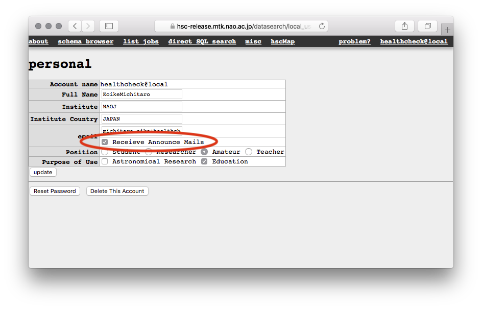
This page does not answer my question. What should I do?
We are sorry about that. Please send your question to hsc_pdr@hsc-software.mtk.nao.ac.jp and we will work on it.