Overview
Processing for HSC SSP data is done using the HSC pipeline, a custom version of the LSST Data Management codebase, specialized and enhanced for Hyper-Suprime Cam processing by software teams at NAOJ, IPMU, and Princeton. Most of the pipeline code was written from scratch for LSST and HSC, with significant algorithmic heritage from the SDSS Photo and Pan-STARRS Image Processing Pipelines. The HSC pipeline can also be used for general-observer HSC or custom processing of SSP data; see documentation for basic installation and use instructions.
There are four major processing stages:
- Single-Visit Processing
- Internal Calibration
- Image Coaddition
- Coadd Measurement
We also have another stage, which is special to this data release only:
- Afterburner Photometry
These steps and output files from there are summarized in the release data page.
Single-Visit Processing (or Single-Frame Processing)
For each CCD in an exposure (“visit”), we:
- Perform low-level detrending: apply bias and flat-field corrections, mask and interpolate defects
- Estimate and subtract the sky background
- Detect and measure bright sources (basic centroiding, aperture photometry, and moments-based shapes)
- Select isolated stars and model the point-spread function (PSF), using a modified version of software developed in a different project (PSFEx)
- Find and interpolate cosmic rays using morphology
- Fit an initial World Coordinate System (WCS) and approximate photometric zero-point by matching to a Pan-STARRS (PS1) reference catalog
- Detect, deblend, and measure faint sources. Includes PSF fluxes as well as several other algorithms that are commonly-used in astronomy
All of the above steps are run separately on each CCD in parallel. We then fit an updated (but not yet final) WCS across all CCDs in an exposure, allowing slight changes in positions and angles of the CCDs within the focal plane.

Internal Calibration (or Mosaic)
Using measurements of stars from the previous stage, we determine final positions and angles of the CCDs and their flux scales. This is done by solving for a final WCS solution with higher-order distortion terms and a spatially-varying photometric zero-point of each CCD, by requiring self-consistent fluxes and centroids for each star.
This procedure is carried out in approximately 1.7×1.7 degree pre-defined areas. These areas are called “tracts” that tile the sky with small overlaps.
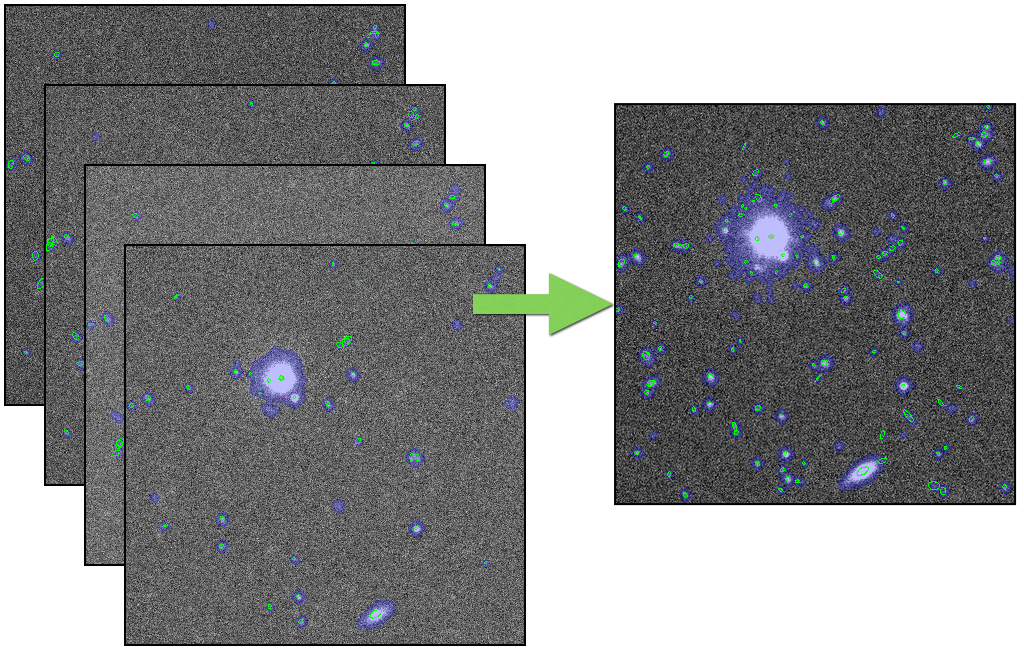
Image Coaddition (or Stack)
All CCD images overlapping a tract are resampled onto a rectangular coordinate system centered on that tract, and then averaged together to build a combined image, called a “coadd”. This is done separately for each band. Instead of matching the PSFs of the input images by degrading images with better seeing, we combine the images as they are, and then construct a PSF model for the coadd image by resampling and combining images of the per-exposure PSF models at the position of every source on the coadd.
To avoid including artifacts (e.g. satellite trails, cosmic rays) or asteroids in the coadd, we actually produce three different coadds. The first is just a simple weighted mean (which does not reject artifacts), and the second uses a sigma-clipped mean (which does). By looking at the difference between these coadds and matching the differences to detections on individual exposures, we can identify these artifacts directly in the original exposures and reject them from final coadd with a simple weighted mean that does not include them. This procedure allows us to reasonably preserve PSFs on the final coadd, while it helps to detect and reject artifacts better than a simple per-pixel outlier-rejection procedure.
Coadd Measurement (or Forced Photometry)
We detect sources on each per-band coadd separately, but before deblending and measuring these sources we first merge them across bands. Above-threshold regions (called “footprints”) from different bands that overlap are combined; peaks within these regions that are sufficiently close together are merged into a single peak. This yields footprints and peaks that are consistent across all bands. We consider each peak to represent a source, and treat all peaks within the same footprint as blended (connecting with neighbor sources).
We then divide (“deblend”) the peaks within the footprints separately in each band. This assigns a fraction of the flux in each pixel to every source in the blend, allowing them to be measured separately. We again run a suite of centroid, aperture flux, and shape measurement algorithms on these deblended pixel values, as well as PSF and galaxy model fluxes and shear estimation codes for weak gravitational lensing.
After measuring the coadd for each band independently, we then select a “reference band” for each source. For most sources, this is the i-band; for sources not detected (or low signal-to-noise) in i, we use r, then z, y, g, and narrow bands. We then perform “forced” measurement in the coadds in all bands, in which positions and shapes are held fixed at their values from the reference band and only amplitudes (i.e. fluxes) are allowed to vary. This consistent photometry across bands produces our best estimates of colors
Afterburner Photometry (or PSF-matched Photometry)
The deblending algorithm used in this data release tends to fail in very crowded areas, such as the central part of a galaxy cluster, resulting in poor photometry. To mitigate the problem, we perform PSF-matched aperture photometry as an afterburner processing. We apply Gaussian smoothing to the coadd images, for three target FWHMs of 0.6, 0.85, and 1.1 arcsec and perform photometry at each target FWHM. In addition to the PSF-matched photometry, the junk suppression algorithm, which was mistakenly disabled in the main processing, is run and objects that should have been eliminated are flagged.